Indefinite Integration of the Gamma Integral
and Related Statistical Applications
3.1 Explaining the "$h$" Function
In the previous section, the discussion of the "$h$" function was restricted to real numbers of the base parameter $s$, except negative integers. This restriction can be relaxed with the following definition of "$h$ ":
\begin{equation*}
h_{s}^{c}=
\begin{cases}
\sum\limits_{i=0}^{\infty }{\frac{{{\left( -c \right)}^{i}}}{\prod\limits_{j=0}^{i}{\left( s+1+j \right)}}}
, &\text{if $s\notin {{\mathbb{Z}}^{-}}$;}\\
{\exp(-c)}\left( \log \left| c \right|+\sum\limits_{s=0}^{\infty }{h_{s}^{-c}} \right), &\text{if $s=-1$;}\\
\sum\limits_{i=0}^{-s-2}{\frac{{{\left( -c \right)}^{i}}}{\prod\limits_{j=0}^{i}{\left( s+1+j \right)}}+\frac{{{\left( -c
\right)}^{-s-1}}}{\prod\limits_{j=0}^{-s-2}{\left( s+1+j \right)}}}h_{-1}^{c}, &\text{if $s\in {{\mathbb{Z}}^{-}}$ & $s\ne -1$.}
\end{cases}
\tag{3.1}
\end{equation*}
[Definition of (3.1)]
When $s$ is not a negative integer, "$h$" is regarded as the core function of the solution to the indefinite
gamma integral. Its asymptotic property at $c\to -\infty$ directly links to the gamma function. When $s$ is a negative integer, "$h$
" is related to the exponential integral, but only in the sense of definite integral. Specifically, we can apply $h_{s}^{c}$ to an
$n$th-order exponential integral with a definite lower and upper limit $a$ and $b$.
\begin{equation*}
\int_{a}^{b}{\frac{{\exp(-x)}}{{x}^{n}}}dx={{{x}^{-n+1}}}{\exp(-x)}h_{-n}^{-x}{\Bigr|}_{a}^{b}
\end{equation*}
The above formula is only meaningful if $a$ and $b$ are positive finite numbers. We can explain why that is the case by discussing the infinite series that defines $h_{-1}^{c}$. As (3.1) makes evident, $h_{s}^{c}$ can be reduced to a function of $h_{-1}^{c}$ when $s$ belongs to negative integers. By definition, $h_{-1}^{c}$ is a two-term product, in which the latter term is the sum of $\log \left| c \right|$ and an infinite number $h_{s}^{-c}$, beginning at $s=0$ and extending to $s\to \infty $. Since all of $h_{s}^{-c}$ are positive when $s\ge 0$, the value of $h_{-1}^{c}$ is contingent on the actual number of terms, noted as "$t$" hereafter, used to compute $\sum\limits_{s=0}^{\infty }{h_{s}^{-c}}$. As a result, its numerical magnitude can not be interpreted directly as the antiderivative value in absolute terms.
When the upper limit is infinity, we encounter a problem in evaluating the asymptotic property of $h_{-1}^{-c}{{|}_{c\to \infty }}$. Fortunately, the finite property of the infinite upper limit applies to all of the "$h$" functions used in calculating $h_{-1}^{-c}{{|}_{c\to \infty }}$. Therefore, the error of replacing the infinite upper limit with a considerably larger number $C$ is trivial.
We refer to two distinct sources of error in applying the "$h$" function to evaluate the exponential integral. The first is the actual number of terms $t$ in the computation of $h_{-1}^{c}$. This is a pure numerical problem, and it is similar to the number of terms from a Taylor series we need to compute an exponential number. The second source of error comes from the evaluation of the "$h$" function when the power parameter $c$ approaches infinity. A discussion of these two kinds of error can be found in Section 4.1 and 4.3.
The functional form of "$h$" does somewhat resembles exp, but "$h$" is not a Taylor series since the denominator is not a factorial term starting from $0!$. If we set $s=-1$, all the denominator terms become $0$ and "$h$" can not be defined by (2.1). Despite their difference, we can easily find certain identities between "$h$" and exp when $s$ is a non-negative integer, such as $h_{0}^{c}={\left[ 1-\exp (-c) \right]}/{c}$.
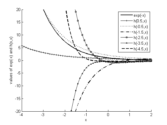
Figure 2: Functional Plots of ${\exp(-x)}$ and $h_{s}^{x}$
Unlike the exponential function, the power parameter $c$ of the "$h$" function takes a negative value in composing the series, and hence, the shape of $y=h_{s}^{c}$ is downward-sloping and decreases to ${{0}^{+}}$ as $c$ increases to infinity, which is similar to the shape of the exponential function $\exp \left( -x \right)$. In addition, the intercept value of the "$h$" function is ${1}/{\left( s+1 \right)}$, and this also differs from the case of the exponential function, which is always one.
Figure 2 presents functional plots of ${\exp(-x)}$ and $h_{s}^{x}$ with six different base parameters. Despite the similar shape, $\exp \left( -x \right)$ intersects with all of the "$h$" functions. This clearly demonstrates that $\exp \left( -x \right)$ and $h_{s}^{x}$ are two distinct functions. When $s>-1$, $h_{s}^{x}$ is a monotonically decreasing function from $x=-\infty $ to $x=\infty$. When $s<-1$, the monotomic increase or decrease of $h_{s}^{x}$ depends on the odd or even number of $\left\lfloor s+1 \right\rfloor $. If $\left\lfloor s+1 \right\rfloor $ is an odd number, $h_{s}^{x}$ is a monotonically increasing function, such as $h_{-1.5}^{x}$ or $h_{-3.5}^{x}$; otherwise, $h_{s}^{x}$ is a monotonically decreasing function, such as $h_{-2.5}^{x}$ or $h_{-4.5}^{x}$
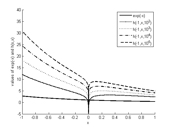
Figure 3: Functional Plots of ${\exp(-x)}$ and $h_{-1}^{x}$ by varying $t$
When $s$ is a negative integer, an $h_{s}^{x}$ function can be represented by an infinite number of curves. Each curve corresponds to a particular number of summation terms $t$ that are used to compute $\sum\limits_{s=0}^{\infty }{h_{s}^{-x}}$ for $h_{-1}^{x}$ in (3.1). As explained in Section 4.3, each curve refers to the same $h_{s}^{x}$ function but with different levels of computational accuracy. Figure 3 presents four indifferent curves of $h_{s}^{x}$ with different levels of precision for one (${{10}^{2}}$), two (${{10}^{3}}$), three (${{10}^{4}}$), and four (${{10}^{5}}$) decimal places. Each set of parentheses contains the number of summation terms $t$ for each curve.
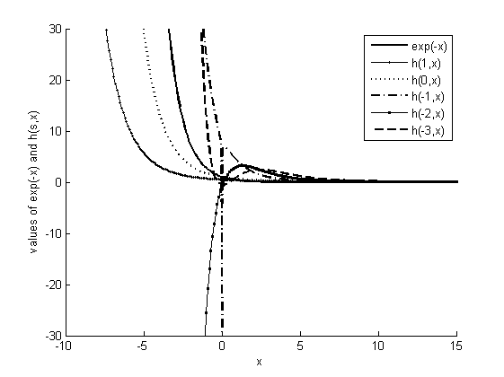
Figure 4: Functional Plots of ${\exp(-x)}$ and $h_{s}^{x}$ with three significant digits (if $s\in {{\mathbb{Z}}^{-}}$)
Maintaining a constant precision level, we can also plot $h_{s}^{x}$ when $s$ is a negative integer. As Figure 4 shows, when the precision level is set to three decimal digits ($t={10}^{4}$), the "$h$" function monotonically decreases if $s$ belongs to non-negative integers or odd negative integers, and it monotonically increases if $s$ belongs to even negative integers. We should be aware that only $h_{-1}^{x}$ has a singular point $x=0$, but the limit of the remaining "$h$" functions does exist and can be evaluated by ${1}/{\left( s+1 \right)}$.
Given that the functional value of "$h$" and the power parameter $c$ have a one-to-one relationship, the inverse function of "$h$", denoted by ${}^{-1}{{h}_{s}}\left( \delta \right)$, can be defined by the following infinite series and is very similar to a logarithmic function:
\begin{align*}
{}^{-1}{{h}_{s}}\left( \delta \right) =&-\left[ \left( s+1 \right)\left( s+2 \right)\delta-\left( s+2 \right) \right] \\ \notag
&+\frac{1}{\left( s+3 \right)}{{\left[ \left( s+1 \right)\left( s+2 \right)\delta-\left( s+2 \right) \right]}^{2}}\\ \notag
&-\frac{s+5}{{{\left( s+3 \right)}^{2}}\left( s+4 \right)}{{\left[ \left( s+1 \right)\left( s+2 \right)\delta-\left( s+2 \right)
\right]}^{3}} \\ \notag
&+\frac{{{s}^{2}}+11s+34}{{{\left( s+3 \right)}^{3}}\left( s+4 \right)\left( s+5 \right)}{{\left[ \left( s+1 \right)\left( s+2
\right)\delta-\left( s+2 \right) \right]}^{4}}+\cdots, \tag{3.2}
\end{align*}
where $\delta=h_{s}^{c}$ and $c={}^{-1}{{h}_{s}}\left( \delta \right)$.
[Proof for (3.2)]
To avoid confusing the inverse sign with the power parameter $c=-1$, we label the inverse function with a left superscript instead of a conventional right superscript. The formula $c={}^{-1}{{h}_{s}}\left( \delta \right)$ in (3.2) can easily be derived from (2.1), and we display the first four terms here. Unfortunately, it usually requires many terms to approximate $c$, and it is more efficient to compute ${}^{-1}{{h}_{s}} \left( \delta \right)$ with iterative methods by numerical analysis. For instance, if we know $h_{1}^{c}=\delta$, the relationship between $c$ and $\delta$ can be specified by (3.1) and reduced to the equation ${{c}^{2}}\delta-c-{\exp(-c)}+1=0$. Solving the equation through a numerical analysis will find the root of $c$, or the value of the inverse function ${}^{-1}{{h}_{s}} \left( \delta \right)$.
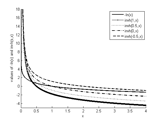
Figure 5: Functional Plots of $-ln(x)$ and ${}^{-1}{{h}_{s}}\left( x \right)$
Figure 5 presents functional plots of $-ln(x)$ and ${}^{-1}{{h}_{s}}\left( x \right)$. Both functions have a similarly shaped curves, but $-ln(x)$ intersects with all the curves of ${}^{-1}{{h}_{s}}\left( x \right)$. Apparently, $-ln(x)$ and ${}^{-1}{{h}_{s}}\left( x \right)$ are distinct functions, too.
Welcome all math lovers!
