Solving Problems in the Panel Regression Model for Truncated
Dependent Variables: A Constrained Optimization Method
4.2 Empirical Findings About Beta Coefficients
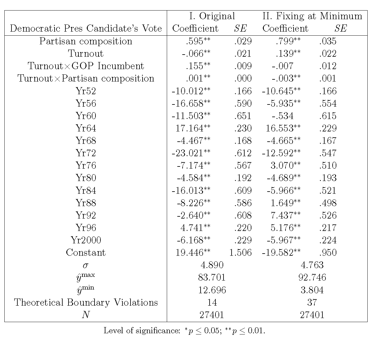
Model I is the original model in which we report all beta coefficients, including the time dummies. We replicate this model using the xtreg command in the Stata environment. The result is presented in Table 2, and we regard this as the base model, since Stata's xtreg command is one of the most widely used methods for panel regression. Due to the nature of the large sample size, all of the beta coefficients are statistically significant at the 0.01 level. Most of the beta coefficients are nearly zero or negative, except Partisan composition, Turnout$\times$GOP Incumbent, Yr64, and Yr96, and the constant.

Table 2 Replication of Table 1 (Column 1) without Constrained Optimization
Hansford and Gomez (2010: 277)
Model II adopts a different specification by fixing all the covariates at the minimum level. In comparing the results of Model I and II, while we expect differences related to the constant and the interaction terms because the model specification changes, the actual difference is far greater than expected. Not only do three of the four main explanatory variables have significant differences, 7 of 13 time dummies also have a different estimate by at least a 3% margin. Moreover, two beta coefficients, Turnout$\times$GOP Incumbent and Yr60, now become insignificant. We reach the same conclusion: different centering specification significantly alters the panel regression results if the model specification involves interaction terms.
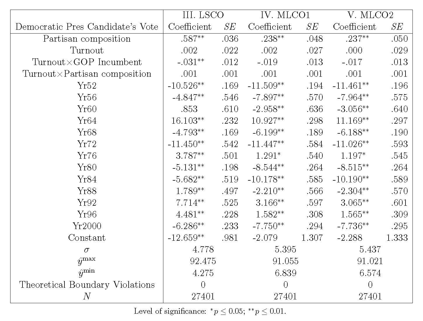
Thus far, we have not applied constrained optimization to the panel regression. In the next three models, we incorporate this nonlinear programming technique under different statistical settings. The first is Model III (LSCO), as reported in Table 3, in which we specify a least squares objective function without any distributional assumption. The model specification is the same as Model II, fixing covariates at the minimum, except that the constant is not comparable given different demeaning operations. We intend to compare Model III with Model II to see how they differ if constrained optimization is applied. The results indicate that the four main beta coefficients have substantial differences, while the time dummies are relatively stable. Specifically, Partisan composition drops .212% from .799% to .587%, and Turnout, Turnout$\times$GOP Incumbent, and Turnout$\times$Partisan composition all have different results of significance.

Table 3 Replication of Table 1 (Column 1) with Constrained Optimization
Hansford and Gomez (2010: 277)
Model IV (MLCO1) is distinct from Model III when taking the distributional assumption into consideration and using the maximum likelihood estimation to form the objective function. The demeaning operation assumes an untruncated normal distribution to the dependent variable. While both models apply constrained optimization, we expect some differences, since the objective function and the parameter set are different. As Table 3 makes evident, the estimated beta coefficients are significantly different. The major difference is not simply the magnitude, but also the level of significance, as well as the sign. For instance, the small change of the beta coefficient is in the Turnout$\times$GOP Incumbent, where the difference is 0.012 when its coefficient is increased from a significant -.031 to insignificant -.019. Considering that the magnitude of the interaction term varies from hundreds to thousands, the 0.012 change is actually quite significant.17 As for the sign of the beta coefficients, 2 of 18 change the sign. This striking difference illustrates the fact that the panel regression under the least squares and maximum likelihood paradigm could generate quite different results with the same model specification.
We further correct the district-level location parameter bias due to the demeaning operation by assuming a truncated normal distribution. Model V (MLCO2) reports the panel regression results with constrained optimization. Comparing Model V and Model IV, their difference is very limited. None of the 18 estimated beta coefficients have a noticeable difference in sign or magnitude, and all of the differences are under the 1% margin. Apparently, the use of the biased estimate, the time mean, to evaluate the district-level properties only causes a marginal difference.
____________________
Footnote
17 We do not mean to evaluate the magnitude of contribution by multiplying an interaction term with the margin of the beta coefficient's change. Since the variation of interaction terms is not independent of its composing variables, we need to incorporate information of other relevant covariates and coefficients to evaluate the actual contribution.
